Understanding the Gini Coefficient: A Measure of Inequality

The Gini coefficient is a crucial statistical tool that quantifies income and wealth inequality within a population. This measure ranges from 0 to 1, where 0 represents perfect equality—indicating that everyone earns the same income—and 1 signifies extreme inequality, where one individual holds all the wealth. Understanding the Gini coefficient is vital for economists, policymakers, and researchers as it provides insights into the economic landscape of nations and communities. The significance of the Gini coefficient extends beyond mere numbers; it reflects social justice, economic stability, and the overall well-being of a population. By comparing income distributions across different countries, the Gini coefficient serves as a lens through which we can analyze socioeconomic conditions. This measure not only highlights disparities but also informs policy decisions aimed at reducing inequality. As global income gaps widen, the importance of the Gini coefficient in economic analysis becomes increasingly apparent, prompting discussions on how to foster equitable growth and development.

Historical Background

The Gini coefficient was introduced by the Italian statistician Corrado Gini in the early 20th century. Gini built upon the foundational work of Vilfredo Pareto, known for the Pareto Principle, and Max Otto Lorenz, who developed the Lorenz curve, which visually represents income distribution. Gini’s contribution was revolutionary, as it provided a concise numerical measure for understanding inequality. However, Gini’s life and work were not without controversy. His political affiliations, particularly with the Fascist regime in Italy, have led to debates about the influence of these beliefs on his statistical work. Despite this controversy, the Gini coefficient has become an essential tool in economic analysis, allowing researchers to discuss income distribution quantitatively. Understanding the historical context of the Gini coefficient enriches our comprehension of its applications and the evolution of inequality measurement over time.

Calculation of the Gini Coefficient

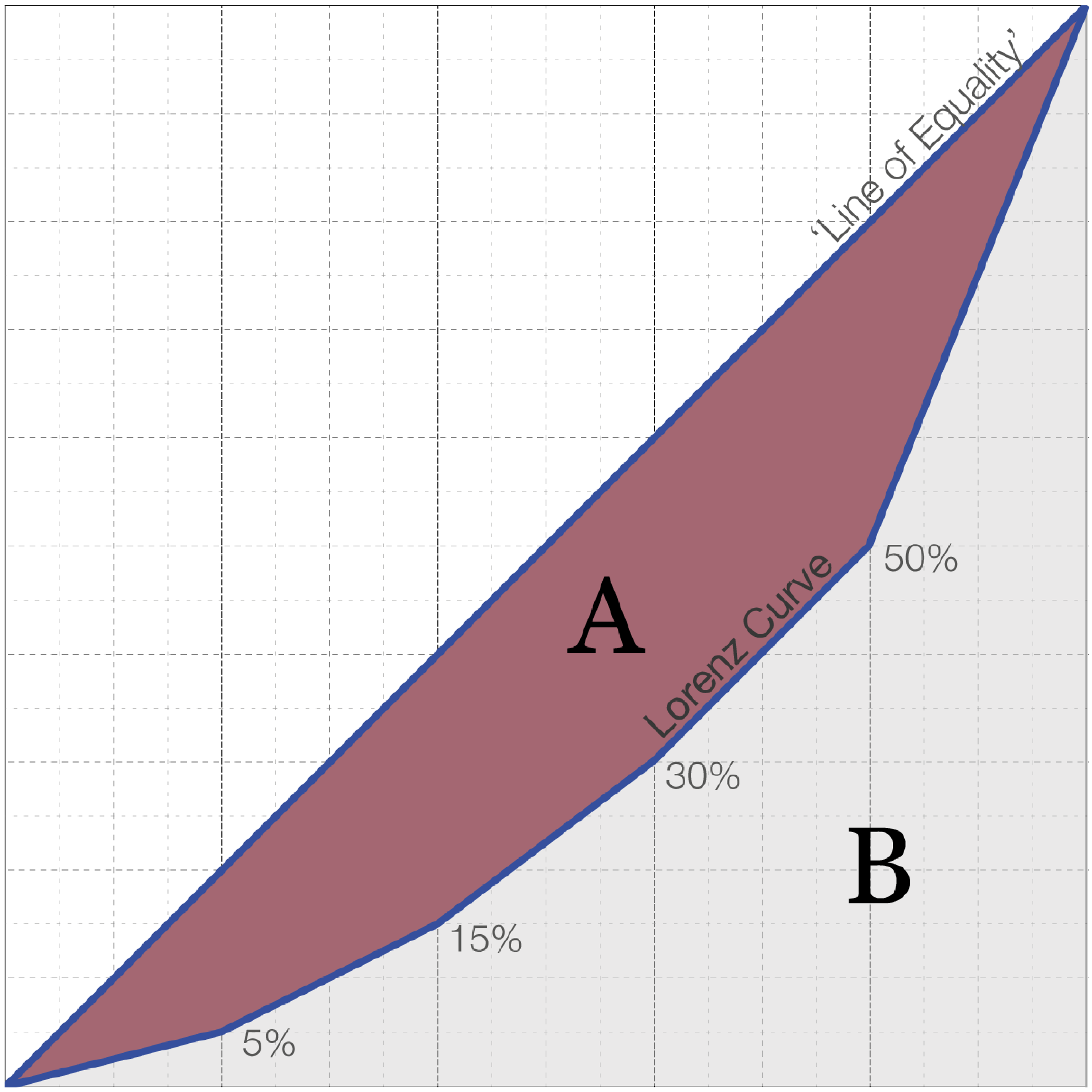
Calculating the Gini coefficient involves a mathematical framework rooted in the empirical cumulative distribution function (ECDF). To derive the Gini coefficient, income data must first be organized in ascending order. This process allows researchers to construct the Lorenz curve, which plots the cumulative share of income received by the bottom x% of the population against the cumulative share of the population. The Gini coefficient is then calculated using the formula: [ G = \frac{A}{A + B} ] Where A is the area between the line of perfect equality and the Lorenz curve, and B is the area under the Lorenz curve. The coefficient can also be interpreted as the ratio of the areas, providing a clear indication of income inequality within a given population. Practical examples highlight how to apply this formula across different datasets, enabling researchers to interpret results meaningfully. Understanding the calculation not only demystifies the Gini coefficient but also emphasizes its importance in economic analysis.

Applications of the Gini Coefficient

The Gini coefficient is versatile and finds applications beyond measuring income inequality. One notable use is in predictive modeling, where it can serve as a correlation coefficient in various fields, including finance and social sciences. By analyzing income distribution patterns, researchers can predict economic trends, assess risk, and inform investment strategies. In finance, the Gini coefficient is often employed to evaluate the distribution of wealth among investors, providing insights into market stability and potential volatility. In social sciences, it helps researchers understand the implications of income inequality on crime rates, education access, and health outcomes. This multifaceted application underscores the Gini coefficient’s significance, making it a valuable tool for economists and policymakers alike. By utilizing the Gini coefficient, stakeholders can make informed decisions aimed at addressing inequality and enhancing societal welfare.

Comparisons with Other Measures of Inequality

While the Gini coefficient is a widely used measure, it is essential to compare it with other statistical tools to gain a comprehensive understanding of inequality. One prominent measure is the Lorenz curve, which graphically represents income distribution. While the Gini coefficient provides a single numerical value, the Lorenz curve allows for a visual interpretation of inequality, making it easier to grasp the concept. Another measure is the area under the receiver operating characteristic (AUC), which is often used in binary classification problems. The AUC assesses the ability of a model to distinguish between different classes, providing insights into predictive accuracy. While the Gini coefficient focuses specifically on income distribution, the AUC measures model performance in various contexts. Understanding these comparisons helps researchers choose the appropriate measure based on the specific analysis, ensuring that economic evaluations are both accurate and relevant.

Global Perspectives on Income Inequality

Examining the Gini coefficient on a global scale reveals stark differences in income inequality among countries. Nations such as Denmark and Sweden typically report low Gini coefficients, reflecting their equitable income distribution. In contrast, countries like South Africa and Brazil exhibit higher Gini values, indicating significant disparities in wealth. These figures have profound implications for social and economic policy. Countries with high Gini coefficients often grapple with issues such as poverty, social unrest, and limited access to education and healthcare. Conversely, nations with lower Gini values tend to experience higher social cohesion and better overall quality of life. Furthermore, correlations between Gini coefficients and other economic indicators, such as GDP per capita, highlight how income inequality can impact economic growth and development. Understanding these global perspectives is crucial for policymakers aiming to foster equitable societies.

Limitations of the Gini Coefficient

Despite its utility, the Gini coefficient has notable limitations. One significant drawback is its inability to capture qualitative aspects of living standards or quality of life. While it provides a numerical representation of income inequality, it does not account for other critical factors such as access to healthcare, education, and social mobility. Therefore, relying solely on the Gini coefficient can lead to an incomplete understanding of economic conditions. Moreover, the Gini coefficient can be misleading when comparing different populations. For instance, two countries may have the same Gini coefficient, yet vastly different economic contexts or cultural dynamics. This highlights the necessity for a comprehensive approach to economic analysis, integrating multiple measures and qualitative assessments to paint a fuller picture of inequality. Recognizing these limitations is vital for researchers and policymakers striving to address income inequality effectively.

Case Studies: Real-World Implications

To illustrate the real-world implications of the Gini coefficient, we can examine case studies from various countries. In the United States, for example, rising income inequality has prompted debates on tax policies and social welfare programs. The Gini coefficient has been instrumental in shaping discussions around economic reforms aimed at reducing disparities. In South Africa, the high Gini coefficient reflects the legacy of apartheid and ongoing socioeconomic challenges. Understanding income inequality in this context has led to policy initiatives aimed at promoting inclusive growth and addressing historical injustices. Scandinavian nations, known for their low Gini values, provide examples of successful social policies that prioritize equality, demonstrating the positive impact of equitable income distribution on societal well-being. These case studies highlight the Gini coefficient’s role in informing policy decisions and its potential to influence economic reforms aimed at reducing income inequality. By analyzing real-world implications, we can better understand how the Gini coefficient shapes discussions around social justice and economic development.

Conclusion and Future Directions

In conclusion, the Gini coefficient serves as a vital tool for understanding income inequality in our world. Throughout this exploration, we have highlighted its significance, historical context, calculation methods, applications, and limitations. The ongoing need for measures that adequately capture economic inequality is evident, as disparities continue to affect societies globally. Looking ahead, the future of the Gini coefficient in economic research appears promising. As new statistical methods and data collection techniques emerge, we can anticipate improvements in the measurement of inequality. Additionally, there is a growing recognition of the importance of addressing qualitative factors that contribute to social and economic disparities. By continuing to explore and address income inequality, researchers and policymakers can work towards creating a more equitable and just world for all.